The Pattern
File structure can be a non-trivial thing in projects. Badly structured projects are confusing—you don’t know what comes from where and can’t tell heads from tails. File names are meaningful, and the folders you put them in are meaningful. In our code, we can create a consistent way to refer to them. This is the focus of this article. I will give a philosophy of file organization, and a specific example that I have used before. It is from a replication assignment, and you can find it here. The example is not intended to be the be-all-end-all of what you should do. Take it more as a guideline for your work.
Data
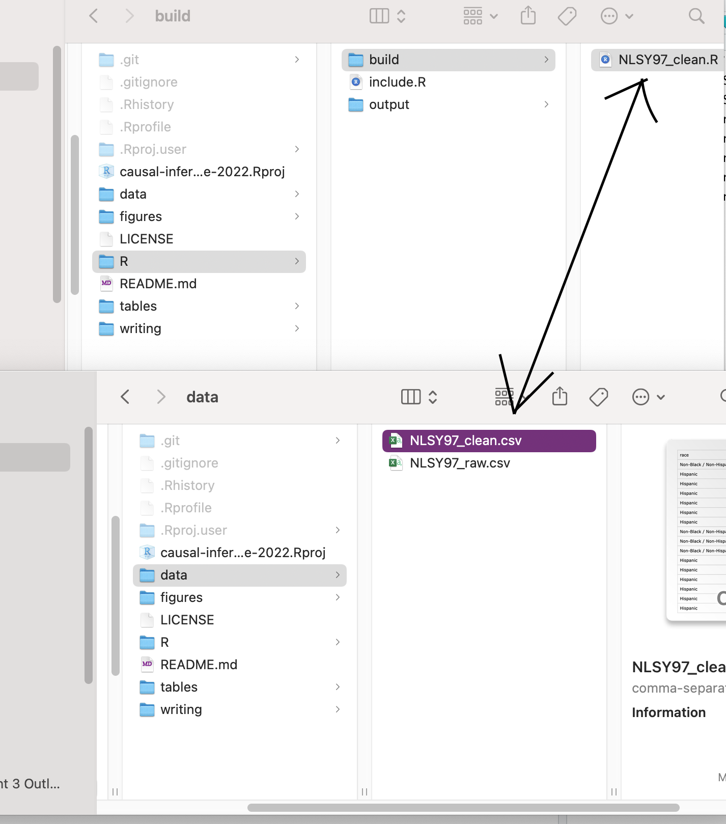
If you’re running a research project, you probably are using some data. If you are using data, you probably will need to clean it somehow. Keep your data in a folder called “data.” If you need to clean it, write an R script inside of a folder called “R” and a subfolder that is reserved for data cleaning/building tasks. In my example below I call this folder “build.”

The name of the R script corresponds to the name of the data set that it cleans. It reads in a “raw” data file, applies whatever transformations are necessary to arrive at a “clean” dataset, and then writes the clean dataset to a new file. The point is to exactly document the steps to get from a dataset that you find on the Internet or in the wild to the dataset that you use in your regressions.
Tables and Figures
If you’re writing a report, you probably have figures and tables that
you need to include. You write R scripts that read in the cleaned data
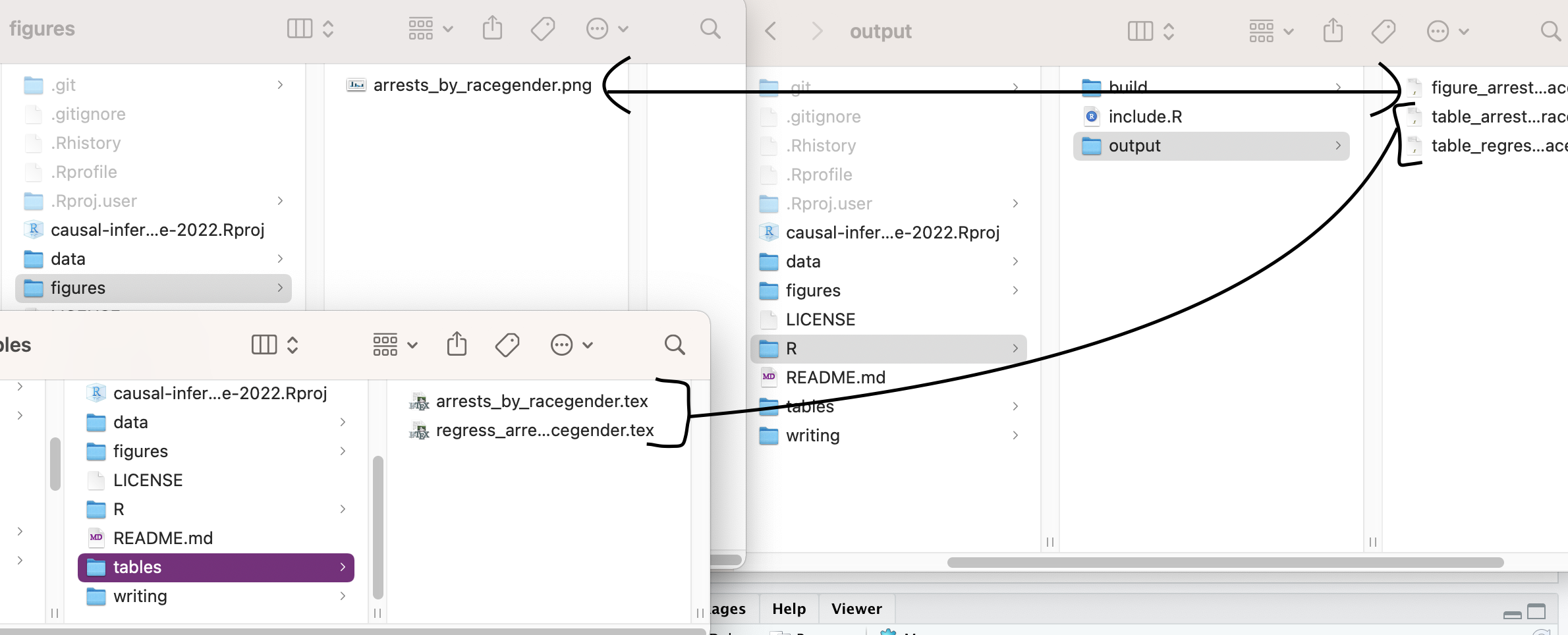
and generate some output as a .png (for figures) or
.tex (for tables). As with data, your figures and tables
live in clearly marked folders. The R scripts that generate the figures
or tables have names that correspond to the figures or tables that they
create. In my example project, I made a subfolder in the R directory
called “output” that has code to generate both tables and figures:
 When you’re creating a figure, you are reading in a cleaned dataset,
possibly doing some cleaning, and then generating a graph. I strongly
recommend using the ggplot2
package. You can then use the
 ggsave() function to write
your graph as a png file.
For tables, you will often have a data frame that represents the
table that you want to put in your paper. The kableExtra
package has utilities to generate a pretty LaTeX table from a data
frame, and then you can write to a file using the tidyverse function
write_lines().
Other times, you may want to output a regression summary into a
table. You can either use the tidy() function from the
broom package to turn your summary into a data frame, and
then follow the kableExtra steps above; or you can use the
stargazer
package to generate pretty regression output. The trade-off between the
two is that because stargazer gives you so much out-of-the-box
functionality, it’s naturally harder to configure it for a very specific
use case.
Where are my files? here they are.
We’ve talked a lot about reading and writing files in this article, so obviously there is a little bit of nuance that I want to impart on you. There are a few different ways that we can refer to files in our code.
The first is an absolute path to our file. This
tells the computer how to find the file from the very top of the
filesystem. For example, a dataset in an R project called “my-project”
would look like
/Users/nate/workspace/my-project/data/some_dataset.csv on
my computer. You can tell a path is an absolute path because it begins
with a forward slash, /. Absolute paths can also start with
a tilde, ~, which indicates that the location is relative
to the home directory of the user. My home directory is at
/Users/nate on my computer, so
~/workspace/my-project/data/some_dataset.csv and
/Users/nate/workspace/my-project/data/some_dataset.csv are
the same thing.
Why are absolute file paths bad? Because they only work on your computer. If some else runs your code, they will have to change the path of the file to wherever their project is located on their own computer. There are better ways to do this. You should avoid absolute paths at all costs, and you will lose points on your assignments if I see an absolute path in your code.
The second way to refer to files is via a relative
path. This tells the computer how to find the file relative to
some folder that I’m currently in. Usually, this is the folder that
holds the R script that is running. Relative paths can be identified
because they start with ./ or ../. If my code
to clean the some_dataset.csv file above lives in
~/workspace/my-project/R/build/some_dataset.R (that is, it
lives inside the “build” folder inside of the “R” folder in my project),
then I can refer to the dataset file in my R code by writing
../../data/some_dataset.csv. That means, “Go up one folder
(to the ‘R’ folder), go up another folder (to the ‘my-project’ folder),
go into the data folder, and find some_dataset.csv there.” Two dots,
../, refers to your script’s parent folder, and one dot,
./, refers to the folder that it is currently in. In most
cases, the one dot can be implicit: hence, my_script.R and
./my_script.R refer to the same thing.
Why are relative file paths bad? They usually do work on multiple
computers because of their relative nature. However, they are prone to
break when you reorganize your code. Say for example that you started
out with all of your code in one R folder, but then later
decide to move your code to multiple subfolders, like
R/build and R/output. When that happens, the
path to your data file is no longer ../data/my_dataset.csv,
it’s now ../../data/my_dataset.csv. To be clear this is not
the worst thing in the world, and relative file paths are acceptable in
many software engineering contexts. For our purposes, we can do better,
though.
The ideal way to refer to files in our projects is via a
project-relative path. This tells the computer, “Look
for the closest .Rproj file, then look relative to that
folder for my file.” This is ideal because it both runs on multiple
computers and is robust to you reorganizing your R scripts. The way we
do this in R is easy. We load the here library, then use
the here() function whenever we refer to a file. So, the
dataset that we have been working with this entire time could be
referred to with here("data/my_dataset.csv"). This may seem
a little abstract, but you can find plenty of usages in my example
project that I linked. One instance is here
in the code for generating a figure.
One thing to keep in mind with here: It is
project-specific. So that means that if you don’t have a project open in
RStudio or you have the wrong project open, then here will
not be able to find your files correctly. If you work with projects the
way that I have suggested you should, this will not be an issue since
you will always have a project open.
Conclusion
Be militant with file naming. Follow a file structure that is
self-evident. This fits perfectly with the “consistent and
predictable” mantra from my meditation on programming. The
here package gives you a consistent and predictable way to
refer to files inside of your project.
Bonus: Build Tools
It is more than enough to make your code so self-evident that someone
else can figure out how to run your scripts and compile your project. To
take it a step further, you can use a build tools such as a Makefile or
a targets file. These are step-by-step recipes of how to
build your projects.
The common vocabulary words that both of these tools use are “target” and “dependency.” A target is something that you want to produce—think of your cleaned dataset, your figure, your LaTeX report. A dependency describes what the target needs to have to run. Build tools track the dependencies so that targets only need to be rebuilt when a dependency changes. This means that you may have many scripts that you need to run that take a long time when all run together, but when using a build tool, it will only build targets for the small parts of the project that actually changed.
Make is a file-based build tool, configured using a file appropriately called the Makefile. Make’s targets and dependencies are specified as files that exist in your project, and Make determines if a target needs to be rebuilt by comparing the last modified time of the target file with the last modified time of all of its dependencies. Make is a concept that almost all software engineers are familiar with, so this is my preferred build tool. The one drawback is that it is file-based, so you inherently have to structure your project so that every target is a file (as opposed configuring targets inside of your R code). A good guide to Make for data scientists can be found here.
An alternative to Make is the targets R package. Instead
of being file-based, you write R code to describe your build process.
targets determines whether a target needs to be rebuilt by
comparing hashes (strings of letter which uniquely identify objects in
code) of the dependencies. It is an interesting concept that I
personally haven’t used in a project yet. You can read about the
targets package here.
Whichever build tool you use, one nice perk is that you can configure the Build tab in the top right-hand corner of RStudio to work with your build tool. In the Build tab, you click the “Build All” button and your project is built! No more having to worry about running scripts in the right order.
If build tools sound good to you, then cool. It’s beyond the scope of this article to go more into depth, but it’s an interesting subject. If you’re my student then feel free to reach out and talk about it.
Happy Coding!